Absenteeism in the Workplace: Preprocessing

Preprocessing Absenteeism data

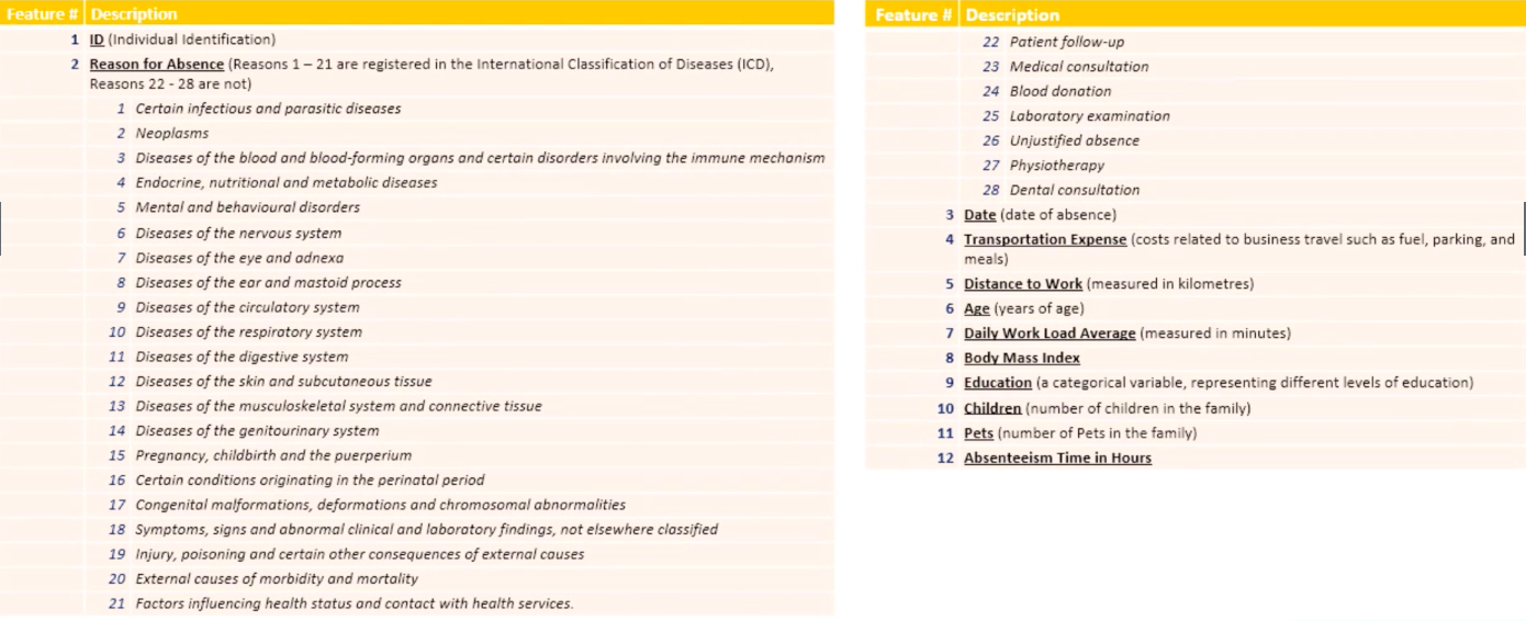
Introduction

In the next FEW articles, we will try to find a solution to Absenteeism in the workplace. More precisely, we would like to find a way to predict when and how long employees can be expected to be away from work.

We will begin by preprocessing our dataset.

Later, we will develop a ML algorithm, the Logistic Regression and analyse the results with the aim of predicting when and why employees typically miss work in a business environment. This helps businesses save money by anticipating absenteeism and deploying measures that minimise the resulting loss in productivity.

Aim

In this exercise, we go through the multiple columns in the dataset and prepare them for the Machine Learning algorithms we will later deploy to find out what intuitions are buried in the data.

The preparation involves extracting relevant data, dropping irrelevant columns and converting the data types in columns to usable format.

The Dataset

The data, and some of the code used in this article are adapted from Data Science Course on Udemy.

The dataset will be uploaded on GitHub on the link below

Loading the dataset:

We begin by importing the relevant libraries: numpy, which allows us to work with numbers and manipulate arrays with ease, and pandas, which is designed for working with panel data.

import numpy as np  # For array manipulation
import pandas as pd # For easily viewing and manipulating dataframes
dataset = '/content/gdrive/My Drive/Colab Notebooks/Absenteeism-data.csv'
raw = pd.read_csv(dataset, sep=',')
raw.head()

Data inspection

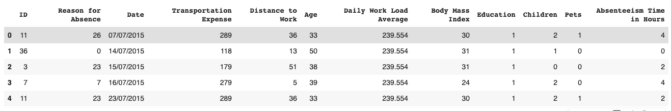
From the file header we see the columns from left to right and data they contain in each row.

A Logistic Regression is an equation of the dependent variable to the predictors/inputs, which are used to predict the target. A logistic regression, for each given row/observation, predicts a binary/ True or False response for the dependent variable. In our case, after preprocessing we will be feeding our regression with the first n-1 columns in order to predict the n$$^{th}$$ column. After eyeballing our columns, we see that the dependent variable we wish to predict is housed in the Absenteeism Time in Hours column at the rightmost end of the columns.

We can also get an initial idea of the dataset by displaying a concise summary of the data contained in each column:

raw.info()

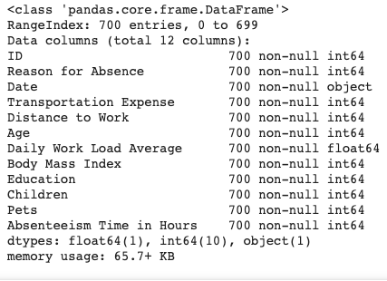This shows us that all the columns have 700 rows of data, as well as the data types, which are mostly 64-bit integers, save for one float column and the Date column, which contains string entries, which in Pandas are referred to as Objects.

Dropping the ID column

From the outset, we can see that the ID column will not be useful for the ML algorithm deployment, since we are not necessarily interested in the individual employees, but their behaviour in general. The ID column distinguishes the observations, but it is in no particular useful order. This nominal variables would actually decrease the predictive power of our resulting algorithm if used in the prediction.

We thus drop this column. But first, let’s save a copy of our raw, unaltered dataframe that we can always revert to in the case of a mistake.

df = data.copy()
df = df.drop(['ID'], axis=1)
print(np.shape(df))

Now, we see that we are dealing with 11 columns containing information relevant to our task. Each of the columns contains 700 observations.

Reason for Absence

This column contains information on the employees’ self-reported reasons for non-attendance.

Let’s take a closer look at this column.

print(df['Reason for Absence'].nunique())

sorted(df['Reason for Absence'])

We see that it contains 28 different reasons for absence from work, from 0 to 28, with reason number 20 missing. Now, can clearly see that these numbers are categorical nominal data points standing for actual reasons for absence. The numbers are obviously used to make the dataset more legible and less voluminous. For our quantitative analysis, we need to understand what these numbers stand for, and rearrange them in a numerically meaningful way for our exercise. One way to do this through dummy encoding.

Dummy Encoding

Dummy variables are a placeholder for categorical variables.

We want to encode the nominal variable Reason for Absence numerically, but without implying some type of ordering.

We thus convert the reason for absence column entries into 0s and 1s. The way to do this is by creating a number of columns corresponding to the number of unique reasons for absence. We then set each observation to 1 for each column to which the reasons correspond.

We create a dummy variables matrix encoding these reasons using pandas:

reason_columns = pd.get_dummies(df['Reason for Absence'], drop_first=True)
print(np.shape(reason_columns))  #700 observations vs 28 reasons for absence.

reason_columns.columns.values

We removed the zeroth dummy variable to avoid multicollinearity issues, using drop_first=True.

Delete Reason for Absence column We drop this column to again avoid multicollinearity issues; we will replace it with the dummy-encoded reasons columns.

df = df.drop(['Reason for Absence'], axis=1)
df.head() # verify the right column has indeed been deleted

Classify the absence reasons into 4 groups:

As can be seen in the feature descriptions above, we can divide the reasons for absence into the following four categories:

• reason 1-14 = various diseases

• reason 15-17 = pregnancies

• reason 18-21 = poisoning-related

• reasons 22-28 = light reasons

reason_1 = reason_columns.loc[:,1:14].max(axis=1)
reason_2 = reason_columns.loc[:,15:17].max(axis=1)
reason_3 = reason_columns.loc[:,18:21].max(axis=1)
reason_4 = reason_columns.loc[:,22:28].max(axis=1)

Now we can put the dummy variables containing all the reasons for absence back into our dataframe.

df = pd.concat([df, reason_1, reason_2, reason_3, reason_4], axis=1)
df.columns.values # Shows that the 4 reasons columns have been appended to the end of the dataframe.  

We must rename the reasons columns to something more descriptive than 0,1,2,3.

The simplest way of achieving this is by copying the column names from the previous Python command and pasting them and manually renaming them before setting the list of column names equal to some variable. This variable is then equated to (thus replacing the value of) the dataframe’s columns, like so:

colnames = ['Date', 'Transportation Expense',
       'Distance to Work', 'Age', 'Daily Work Load Average',
       'Body Mass Index', 'Education', 'Children', 'Pets',
       'Absenteeism Time in Hours', 'reason_1', 'reason_2', 'reason_3', 'reason_4']
df.columns = colnames

We still need to move the reason columns to the position where we removed the original Reason for Absence column. Again, we do this manually:

cols_reordered = ['reason_1', 'reason_2', 'reason_3', 'reason_4', 'Date', 'Transportation Expense', 'Distance to Work',
                     'Age', 'Daily Work Load Average', 'Body Mass Index', 'Education', 'Children', 'Pets', 'Absenteeism Time in Hours']
df = df[cols_reordered]

At this point, we have repositioned the reasons for absence at the beginning of the columns list in the data frame.

The Date Column

The next column to handle is the Date column.

print(df_reason.Date.head())
df_reason.Date.dtype

The date column’s entries are strings. Let’s convert these dates from string to the datetime format, also known as a Timestamp:

df_reason.Date = pd.to_datetime(df_reason.Date, format='%d/%m/%Y')

This changes the datatype of the observations in this column from Objects (the pandas name for strings) to 64-bit datetime entries.

Now, we would like to understand the monthly and weekly trends in absenteeism. We would thus like to extract the month value from each date entry:

df_reason.Date[1], df_reason.Date[1].month
>> (Timestamp('2015-07-14 00:00:00'), 7)

The second (arbitrary example) entry has a date of 14 July 2015. We extract the month value by appending .𝚖𝚘𝚗𝚝𝚑 to the end of the Timestamp Let’s extract the month values and make a separate column for them

months = []
for i, j in enumerate(df_reason.Date):
  months.append(j.month)

Let’s put these month values in the dataframe

df_reason['Month'] = months

We can similarly extract the day of the week. NB: Due to Python’s zero-indexing, the first weekday, Monday has an index of 0, and the final day of each week, Friday, has an index of 4.

day = []
for i, j in enumerate(df_reason.Date):
  day.append(j.weekday())
df_reason['Day of the Week'] = day

Now that we got all the information we need from the date column, we can drop that column and them move the month and weekday column to replace it.

df_reason = df_reason.drop(['Date'], axis=1)
df_reason.columns.values

colnames = ['reason_1', 'reason_2', 'reason_3', 'reason_4', 'Month',
       'Day of the Week', 'Transportation Expense', 'Distance to Work',
       'Age', 'Daily Work Load Average', 'Body Mass Index', 'Education',
       'Children', 'Pets', 'Absenteeism Time in Hours']
df_reason = df_reason[colnames]

Education Column

The next column we consider is the Education column.

df_reason_date['Education'].unique(), df_reason_date.Education.nunique()

How are the different education levels represented in our data sample?

df.Education.value_counts().plot('bar')
plt.xlabel('1=High school, 2=undergrad, 3=postgrad, 4=MSc/PhD')
plt.title('Education Level Counts')
plt.ylabel('Counts')
plt.savefig('education.png', figsize=(16, 12), dpi=80)
plt.show()

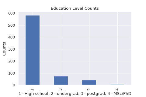
The majority of the people surveyed have a high school education, followed by postgraduates (Honours) and then undergraduates and MSc/PhD holders, in that order.

Since the number of high-school graduates is much higher than the tertiary educated counts, we lump all the tertiary educated observations together:

0 – high school

1 – tertiary

df_reason_date.Education = df_reason_date.Education.map({1:0, 2:1, 3:1, 4:1})
100*sum(df_reason_date.Education)/len(df_reason_date.Education)

Only 16.71% of the surveyed observations have a tertiary education. We will later investigate how education level relates to absenteeism.

That’s it! For now we can take this to be our full preprocessed data set.

After saving the preprocessed dataframe in a variable, the next thing to do is create a ML model to look for trends in the data that can explain why and when absenteeism occurs in the workplace, as well as who typically absconds

df_preprocessed.to_csv('absenteeism_data_preprocessed.csv', index=False)