Machine Learning Project: Wine Data Set

Using Machine Learning to classify red wine

For Data Science or Wine enthusiasts: Read this to see how we can predict the quality of red wine using Data Science and some information on the ingredients of the wine.

Dataset:

The dataset, which is hosted and kindly provided free of charge by the UCI Machine Learning Repository, is of red wine from Vinho Verde in Portugal.

In a Google Colab/Kaggle/Jupyter notebook, We load a csv file containing our dataset from the UCI ML repository and quickly view our dataset like so:

Loading the dataset

import numpy as np  # For array manipulation
import pandas as pd # For easily viewing and manipulating dataframes
dataset_url = 'http://mlr.cs.umass.edu/ml/machine-learning-databases/wine-quality/winequality-red.csv'
data = pd.read_csv(dataset_url, sep=';')
data.head()

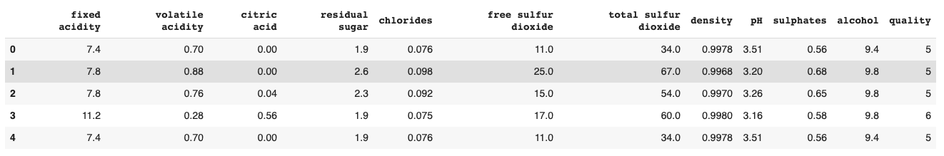
Here we see the first a bunch of labeled columns, from fixed acidity to quality, and the first 5 rows of the dataset.

Aim:

We want to predict the quality of red wine given the following attributes:

• fixed acidity
• volatile acidity
• citric acid
• residual sugar
• chlorides
• free sulfur dioxide
• total sulfur dioxide
• density
• pH
• sulphates and
• alcohol

Exploratory Data Analysis

Let’s take a closer look at the dataset. We start by separating the target column, which contains the wine quality information, from the features:

target = data.quality # The targets column
X = data.drop('quality', axis=1) # features

print('\nOur data has %d observations and %d features\n' %(X.shape[0], X.shape[1]))

#columns with missing data
print('Are there missing observations the columns?\n', (data.isnull().any()))

print('\nThere are', target.nunique(), 'Unique values for quality, namely:', sorted(target.unique()))

We see that our data has 1599 observations and 11 features. None of the columns contain any missing variables, which makes our task a lot easier.

The target.nunique() and target.unique commands give us the number and values of all the unique entries in the target column. We see that our data contains 6 wine qualities: 3, 4, 5, 6, 7 and 8.

How are the 1599 wines distributed in quality?

vgq = data[target>6]  #top tier quality
aq = data[(target>=5) & (target<=6)]  #average quality
bq = data[target<5]   #bad quality

print('%.2f %% of the wines are of top tier quality' %(100*len(vgq)/len(target)))
print('%.2f %% of the wines are of average quality' %(100*len(aq)/len(target)))
print('%.2f %% of the wines are below average quality' %(100*len(bq)/len(target)))

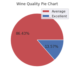
13.57% of the wines are are of top tier quality, i.e they have a quality of 7 or 8. The bulk ( 82.49% ) of the wine is of comparatively average quality while 3.94% are below average in quality.

Numbers are cool, but graphics make more sense to most of us. What does the wine quality distribution look like in a ~histogram~ bar graph?

import matplotlib.pyplot # The go-to library for plotting in python
import seaborn as sns # Another powerful library for pretty and useful visualisations
sns.set() #initialise seaborn so that all our plots are exciting by default


sns.distplot(target, norm_hist=False, kde=False)
plt.title('Wine quality feature distribution')
plt.ylabel('Number of observations')
plt.show()

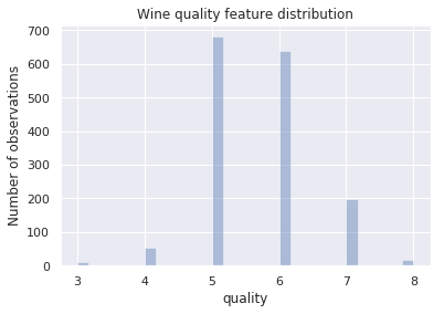
“That’s what I do, I drink and I know things” - Tyrion Lannister

We see from the bar graph that indeed most of the wines are of average quality, less than half are above average while even fewer are below average.

However, we are interested in the excellent quality wines. Let’s therefore separate the wines of excellent quality ( \geq 7 ) from the rest. We will be building classifiers, given the 11 features, that separate/identify excellent quality wine from the rest.

Let’s begin by creating a column of binary values in the features dataframe X, which indicates whether the wine is of excellent (1) or less than excellent quality (0):

XX = X.copy() # To be safe, let's only modify a copy of the features DF

XX['best_quality'] = 1
XX['best_quality'][target<7] = 0 # All wines less than excellent

XX.describe()

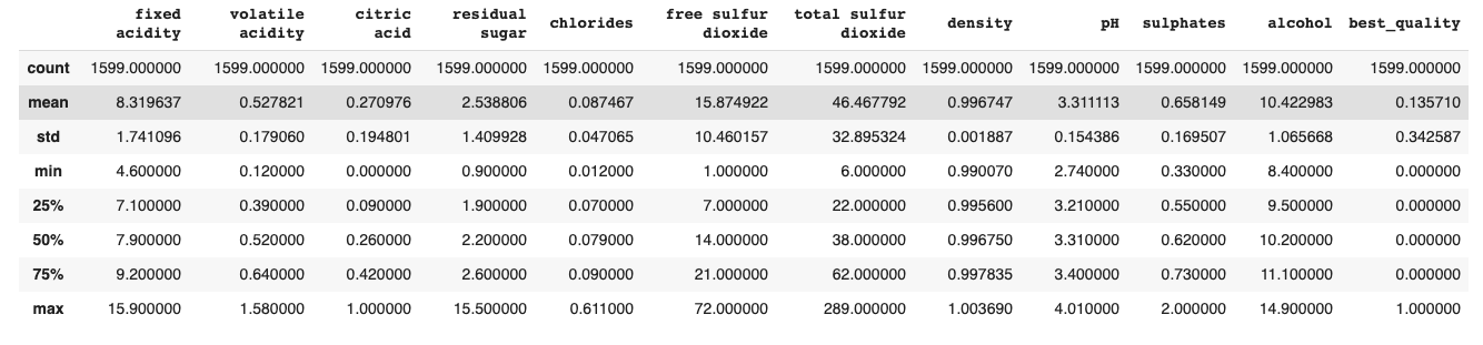
The XX.describe command gives us a summary of the statistics of each column in XX.

Now we have only two classes of wine. This pie chart shows us how our raw data is distributed in wine based on the two classes we defined:

plt.pie(XX.best_quality.value_counts(), autopct='%1.2f%%', colors=['r', 'b'])
plt.legend(labels=['Average', 'Excellent'], loc='best')
plt.title('Wine Quality Pie Chart')
plt.show()

Our problem is thus:

Given the features in XX.columns.values, we want to predict whether or not a wine will be of excellent quality

We thus redefine our targets and features:

# The targets are now composed of 2 classes (excellent and not excellent)
y = XX.best_quality
# Let's drop the targets column from the features dataframe
XX = XX.drop(['best_quality'], axis=1)

Before we proceed to the next step, Let’s have a look at the correlations between our features

The features we train our data on should not be too correlated with each other, to avoid Multicollinearity, a key assumption in Linear Regression analysis which could also be an issue in Classification problems

correlation = data.corr()
plt.figure(figsize=(14,12))
plt.title('Correlation')
sns.heatmap(correlation, annot=True, linewidths=0, vmin=-1, cmap="RdBu_r")
plt.show()

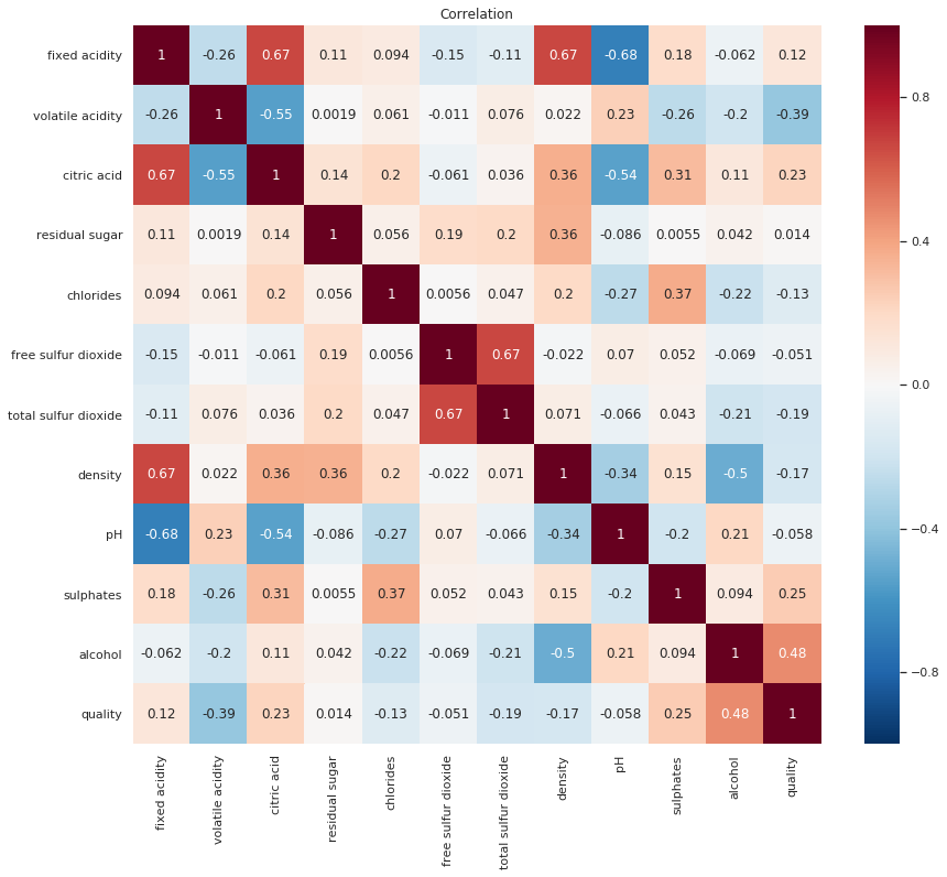
There is no consensus on what the correlation threshold for multicollinearity should be, and thus this might just be down to trial and error.

We will first train our models with all the features and later check if we can somehow increase model accuracy by addressing the highest correlations.

Preprocessing

Train-test-split

We must split our data into a training set and a validation/test set. The test set is set to be a small fraction of the observations, and the rest is used for training. The train_test_split module from scikit-learn does just that job for us. specifying the test size automatically tells train_test_split to make the remaining data the training set, and vice-versa.

from sklearn.model_selection import train_test_split

X_train, X_test, y_train, y_test = train_test_split(XX, y, test_size=0.25,
                                                   random_state=0, stratify=y)

Do we have any categorical variables in our features?

cat = [cname for cname in XX.columns if XX[cname].dtype=='object']
print('There are %d columns with categorical entries\n' %len(cat))

Raw data usually comes with a lot of missing, unreliable entries, as well as data of different types. We ideally want all our data to be numerical, and at the same scale, for comparability. Since our data contains no missing or categorical values (phew!), the entire Preprocessing process will entail standardizing the data. We do this, for each column, by taking each observation X and transforming it according to: \(z = \frac{X-\mu }{\sigma}\)

In this case we are going to perform all the preprocessing inside the ML models’ pipelines. Speaking of which…

Models

We will try multiple ML classifier algorithms and evaluate their performance to select the best model for our problem.

We will try training the following algorithms on our data:

• A Decision Tree Classifier

• A Random Forest ensemble Classifier and

• the eXtreme Gradient Boosting Classifier.

from sklearn import preprocessing

print('Defining the Classifiers and fitting them on our training data...')

decTree_pipeline = Pipeline(steps=[('preprocessor', preprocessing.StandardScaler()),
                                   ('model', DecisionTreeClassifier(random_state=0))])
decTree_pipeline.fit(X_train, y_train)

RF = Pipeline(steps=[('preprocessor', preprocessing.StandardScaler()),
                     ('model', RandomForestClassifier(n_estimators=1000, random_state=0))])
RF.fit(X_train, y_train)


xgb = Pipeline(steps=[('preprocessor', preprocessing.StandardScaler()),
              ('model', xgboost.XGBClassifier(n_estimators=1000, learning_rate=0.05))])
xgb.fit(X_train, y_train)

print('...\nDone!')

Here we defined simple pipelines for each of our candidate models. In each pipeline we specify the basic preprocessing required, which is simply a StandardScaler from the scikit-learn library’s preprocessing module, then specified the model names, with mostly the default settings. The random_state allows us to seed the classifiers’ randomness such that subsequent runs and checks will reproduce the same result unless the random_state is changed to another value. The learning_rate, simply put, is the step size, which allows the model to better converge to the ‘correct’ answer (a minimum of the loss function, which we typically want to minimize) when set to a low enough number, though when too small it leads to a much slower convergence of the model. n_estimators refers to the number of trees used in the random forest algorithm, which itself is an ensemble of decision trees.

Model predictions

After training our 3 model pipelines on the training feature set, we can now use the test features to make predictions for each model.

tree_pred = decTree_pipeline.predict(X_test) #decision tree
rf_pred = RF.predict(X_test) #random forest
xgb_pred = xgb.predict(X_test) #xtreme gradient Boosting

Evaluating Classifier performance

Naturally, we proceed to ask: how well do these predictions match the actual test targets?

Classification Accuracy

What percentage of the predictions made by each model were correct? classification accuracy provides this answer by simply comparing the test targets to each of the predicted targets.

In Python:

from sklearn.metrics import accuracy_score

print ('Accuracy: Decision Tree = %s%%' %(100*accuracy_score(y_test, tree_pred)))
print ('Accuracy: Random Forest = %s%%' %(100*accuracy_score(y_test, rf_pred)))
print ('Accuracy: xg boost = %s%%' %(100*accuracy_score(y_test, xgb_pred)))

We get an accuracy score of 89.25% for the Decision Tree Classifier, 90.25% for the Random Forest classifier and 91.0% for the Xtreme Gradient Boosting classifier. All these values seem quite impressive. The XGB is clearly the winner in this instance, but let’s invesitage further…

Null Accuracy

This is the accuracy we would get if we just let the classifier always predict the most common class every time. i.e If we let our classifier claim that all the wines are not excellent, how accurate would it be?

print('A model that always predicts insipid wine quality would be\
 accurate\n %.2f%% of the time' %(100*(1-y_test.mean())))

Since only 13.57% of the observations (wines considered in the dataset) are of excellent quality, We get a null accuracy of 86.50%.

The Confusion Matrix

• describes a classification model’s performance by comparing the predicted classes to the expected classes.

from sklearn.metrics import confusion_matrix

print('Confusion Matrix for simple, gradient boosted, and random forest tree classifiers:')
print('Simple Tree:\n',confusion_matrix(y_test,tree_pred),'\n')
print('Gradient Boosted:\n',confusion_matrix(y_test,rf_pred),'\n')
print('Random Forest:\n',confusion_matrix(y_test, xgb_pred))

output:

Confusion Matrix for simple, gradient boosted, and random forest tree classifiers:
Simple Tree:
 [[324  22]
 [ 21  33]]

Gradient Boosted:
 [[331  15]
 [ 24  30]]

Random Forest:
 [[327  19]
 [ 17  37]]

The rows represent the actual (True) classes while the columns represent the predicted classes. This is helpful, but we could display this much better using heatmaps from seaborn.

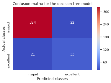
Example, for the decision tree classifier:

ax = plt.subplot()
sns.heatmap(confusion_matrix(y_test, tree_pred), annot=True, fmt='d', cmap='coolwarm')
ax.set_xlabel('Predicted classes')
ax.set_ylabel('Actual classes')
ax.xaxis.set_ticklabels(['insipid', 'excellent'])
ax.yaxis.set_ticklabels(['insipid', 'excellent'])
plt.title('Confusion matrix for the decision tree model')
plt.show()

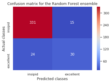
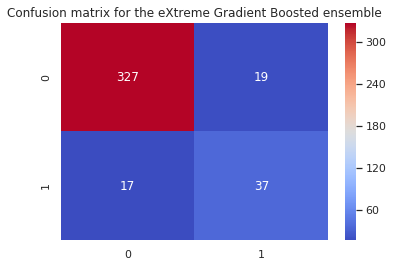
For the random forest classifier:

and for the XGBoost:

Furthermore, we can summarise the performance of each model in a Classification Report:

from sklearn.metrics import classification_report

print(classification_report(y_test, tree_pred))

and so forth for the other 2 models.

The output is thus:

For the DecisionTreeClassifier

precision    recall  f1-score   support

0       0.94      0.94      0.94       346
1       0.60      0.61      0.61        54

accuracy                           0.89       400
macro avg       0.77      0.77      0.77       400
weighted avg       0.89      0.89      0.89       400

For the RandomForestClassifier

precision    recall  f1-score   support

          0       0.93      0.96      0.94       346
          1       0.67      0.56      0.61        54

   accuracy                           0.90       400
  macro avg       0.80      0.76      0.78       400
weighted avg       0.90      0.90      0.90       400

And for the XGBClassifier

precision    recall  f1-score   support

          0       0.95      0.95      0.95       346
          1       0.66      0.69      0.67        54

   accuracy                           0.91       400
  macro avg       0.81      0.82      0.81       400
weighted avg       0.91      0.91      0.91       400

The model comparison is clear, compact and concise. Classification report allow us to evaluate and compare a lot of information in a concise manner.

We can still proceed to use the ROC curve to visualise and find a balance between sensitivity and specificity, as our needs require..

We use probabilistic predictions here, instead of the actual predictions made by our models…

tree_pred_prob = decTree_pipeline.predict_proba(X_test)[:,1]
rf_pred_prob = RF.predict_proba(X_test)[:,1]
xgb_pred_prob = xgb.predict_proba(X_test)[:,1]

Generating and plotting the ROC curves:

from sklearn.metrics import precision_recall_curve, roc_curve

fp_tree, tp_tree, thresh_tree = roc_curve(y_test, tree_pred_prob)
fp_rf, tp_rf, thresh_rf = roc_curve(y_test, rf_pred_prob)
fp_xgb, tp_xgb, thresh_xgb = roc_curve(y_test, xgb_pred_prob)

plt.plot(fp_tree, tp_tree, 'r--', label='Tree')
plt.plot(fp_rf, tp_rf, 'g-', label='Forest')
plt.plot(fp_xgb, fp_xgb, 'b--', label='XGBoost')
plt.title('ROC Curves for the three models')
plt.xlabel('False Positives Rate (= 1 - specificity)')
plt.ylabel('True Positives Rate (= sensitivity)')
plt.legend(loc='best')
plt.show()

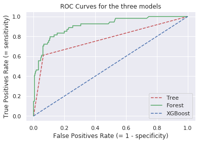
What we are actually interested in is the Area Under the Curve for each of the classifiers. Since we are interested in identifying the best quality wines, we are trying to optimise our models for the detection of true positives.

import roc_auc_score
print('Decision Tree AUC:\t %.2f%%' %(100*roc_auc_score(y_test, tree_pred_prob)))

print('Random Forest AUC:\t %.2f%%'  %(100*roc_auc_score(y_test, rf_pred_prob)))

print('XGBoosting AUC: \t %.2f' %(100*roc_auc_score(y_test, xgb_pred_prob)))

The AUC for the three algorithms is: DTC = 77.38%, RFC = 90.80 and XGBoost = 90.21.

We have a clear winner, the Random Forest Classifier!

Going forward, we must optimise the RF to get the best possible predictions from it. But first, let’s see if TPOT can’t do much better.

TPOT is a Python-based Automated ML tool that uses genetic programming to find the best model, pipeline and hyperparameters for a given dataset.

On Google Colab, you can quickly install TPOT in the current notebook and import the classifier by running:

!pip install tpot
from tpot import TPOTClassifier

Then we let it search for the optimal pipeline:

tpot =  TPOTClassifier(generations=10, population_size=20, verbosity=3, n_jobs=-1)
tpot.fit(X_train, y_train)
print(tpot.score(X_test, y_test))

The arguments of TPOTClassifier may be tinkered with depending on your needs, patience and computing power. n_jobs=-1 allows TPOT to parallelize to all usable nodes, while the other 3 arguments are generally better when set to bigger values, again, given that you are very patient and using a reliable machine.

To export the final pipeline obtained by TPOT:

tpot.export('tpot_wine_pipeline.py')
!cat tpot_wine_pipeline.py #display the final pipeline

Compare the resulting pipeline with the defending champion for this dataset, the RFC. We get the tpot predictions by running

tpot_preds = tpot.predict(X_test)

Stay in touch for more data science hijinks!